neuralign
All things neural distribution alignment
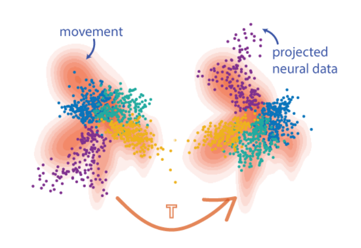
Dimensionality reduction is a powerful tool to analyze neural activity at the population level. However, a number of considerations - including the non-uniqueness of low-dimensional representations, instabilities in recording, and biological factors like plasticity - can cause the latent representations of two recordings, which should be similar enough to be directly comparable, to differ by a transformation. The objective of neural distribution alignment is to recover and invert this transformation, so that we can robustly compare neural activity across time, space, and even subjects.
We provide here open-source access to two algorithms designed to tackle this problem: Distribution Alignment Decoding, which uses a brute-force approach to find the optimal transformation; and Hierarchical Wasserstein Alignment, which exploits the tendency of neural distributions to be composed of clusters to find the solution more elegantly. Find below implementations in MATLAB and the Python scientific stack, as well as some sample datasets.
Distribution Alignment Decoding for Neural Data
Eva Dyer et al., A cryptography inspired approach for movement decoding, Nature BME, 2017.
Hierarchical Wasserstein Alignment (HiWA)
John Lee, Max Dabagia, Eva Dyer, Chris Rozell: Hierarchical Optimal Transport for Multimodal Distribution Alignment, to appear at NeurIPS 2019.
nBME Comment: Comparing high-dimensional neural recordings by aligning their low-dimensional latent representations
Why alignment?
Systems neuroscience is currently experiencing a renaissance. Over the past decade our neural recording capabilities have expanded tremendously, and it is now possible to capture the activity of hundreds to thousands of individual neurons simultaneously. The most promising approach to analyzing datasets of this size is to distill the activity of many neurons down to a smaller number of explanatory latent variables. This is usually accomplished by means of the many dimensionality reduction techniques developed in the machine learning community, as well as more specialized variants designed to exploit the temporal properties of dynamical systems. With suitable latent representations for neural activity, we can compare different neural recordings, even if they were made at different times, recorded different groups of neurons, or even came from different subjects.
However, many dimensionality reduction techniques, especially nonlinear ones, are not guaranteed to yield unique latent variables. Even when exactly the same information is encoded in multiple recordings, the resulting latent spaces may differ from each other by an invertible transformation. Furthermore, whenever we try to compare multiple recordings, we implicitly make the assumption that our sample of neurons in the population is sufficiently diverse; that is, uncorrelated enough so it fully captures the key dynamical processes of the circuit, yet not so uncorrelated that we end up sampling the behavior of multiple circuits, each of which operates nearly autonomously. At present, it is not well understood how to choose neurons to ensure these properties, or even how large a sample needs to be when neurons are selected at random. When the latent space is sufficiently simple, and each variable comprising it corresponds roughly to a trend in activity among some neurons, single units can be found whose activity patterns roughly correspond to the leading principal components of the entire population. However, in unsupervised sampling procedures the low dimensional structure easily breaks down, since even if the right neurons are chosen a single high-variance unit can obfuscate the the rest.
The distribution alignment problem has received some attention in machine learning, where identifying shared structure across datasets is a critical objective in the unsupervised and transfer learning paradigms. We recently introduced a few different approaches, tailored to the neural decoding setting. The first, Distribution Alignment Decoding (DAD), uses density estimation to infer the probability distributions in latent space, and then, owing to the non-convexity of Kullback-Leibler divergence, employs a brute-force search to identify the optimal rotation which matches the two distributions. The second, Hierarchical Wasserstein Alignment (HiWA), improves upon this strategy by using the structure of the data to decompose the alignment problem, namely the tendency of neural circuits to constrain their low-dimensional activity to clusters or low-dimensional subspaces. In conjunction with a more geometric formulation of distance drawn from optimal transport, HiWA is able to more quickly and robustly recover the correct rotation.
The ability to robustly find common latent spaces for neural recording has several applications. In an exploratory context, it allows us to understand how neural encoding strategies change over time or as the subject enters different states, such as wakefulness or attention. With labelled data, we can even use it to perform unsupervised decoding in a form of transfer learning, by mapping labelled and unlabelled datasets into the same space, and then classifying unlabelled points based on the labeled points they are close to.
The Algorithms
DAD was significant because it proved that unsupervised decoding for brain-machine interfaces is possible through the combination of dimensionality reduction and distribution alignment. However, it is included here mostly for historical purposes; it uses a fast algorithm to perform estimate probability density from the samples, but this is still slower than no density estimation at all, and then due to the non-convexity and poor behavior of KL divergence between distributions with differing support, has to resort to a brute-force search of possible rotations to find the right one.
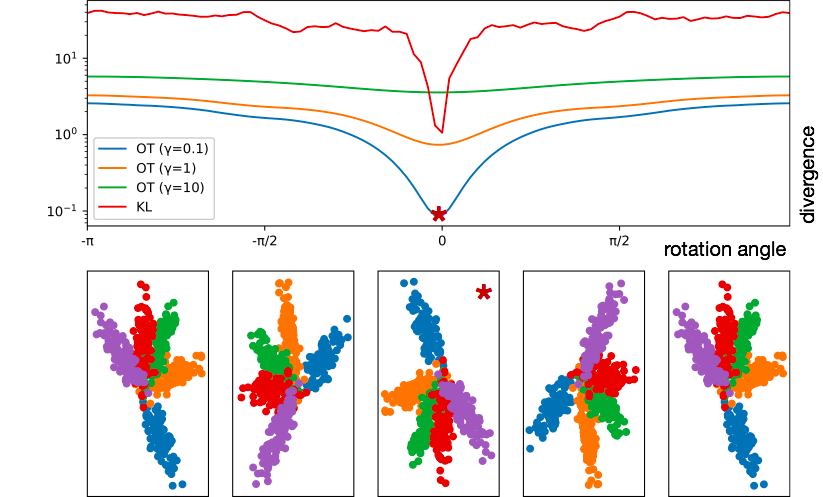
In constrast, HiWA leverages computational optimal transport to make use of a more geometrically sensical notion of distance, which typically smoothly decreases as one gets closer to the correct rotation. It also takes advantage of clusters in the dataset to decompose the non-convex alignment problem into several smaller and easier cluster-wise alignment problems, which generally adds strong convexity and allows the algorithm to run mostly in parallel.
Below, we demonstrate how KL and Wasserstein divergence stack up; Wasserstein divergence is shown as the strength of the entropy relaxation applied to it is varied.
Contributers
This project was developed by Max Dabagia and Eva Dyer, in NerDSLab at Georgia Tech.